Logistic Regression was invented in 1958. It’s the “Hello World” of machine learning—the algorithm every data science student learns first and then forgets about.
So when I decided to test it against real network intrusion data—25,000 connections containing SYN floods, buffer overflows, port scans, and password brute-force attacks—I expected it to fail.
It didn’t. But it failed in ways I didn’t expect.
I’m an offensive security engineer. I’ve exploited web apps, escalated privileges, and simulated red team operations. But I’d never seriously looked at the detection side—the algorithms that are supposed to catch people like me.
This article is what I found when I did.
The Dataset That Doesn’t Play Fair
Most ML tutorials use clean, well-behaved datasets. The NSL-KDD dataset is not one of them.
It was built by MIT Lincoln Labs to simulate a military network under attack. Each record represents a single network connection described by 41 features—things like protocol type, bytes transferred, error rates, and login attempts.
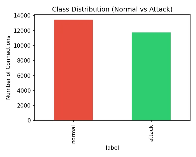
The training set contains 25,192 connections with 22 known attack types across four categories:
- DoS—SYN floods, smurf attacks
- R2L—Remote password guessing, unauthorized access
- U2R—Buffer overflows, rootkit installations
- Probing—Port scanning, network surveillance
But here’s what makes this dataset brutal: the test set contains 14 attack types that don’t exist in the training data.
Read that again. The model is evaluated on attacks it has literally never seen before. This is not a toy benchmark—it mirrors the reality that attackers constantly evolve their techniques.
Version 1: Give the Model Everything
The Setup
41 features. Three of them are categorical (protocol_type, service, flag), so they need to be converted to numbers via one-hot encoding. This expands the feature space to 118 columns.
Standardize everything. This is critical because features like src_bytes can reach millions, while others like serror_rate are bounded between 0 and 1.
Without scaling, the model becomes dominated by large-magnitude features—not because they’re more important, but simply because of their scale. Standardization ensures each feature contributes proportionally to the model.
Train a Logistic Regression model on the standardized data, then evaluate its performance on a separate test set to measure how well it generalizes to unseen network traffic:
# One-hot encode categorical variables
X_train = pd.get_dummies(df.drop("label", axis=1),
                         columns=["protocol_type", "service", "flag"])

# Standardize - without this, the model barely converges
scaler = StandardScaler()
X_train_sc = scaler.fit_transform(X_train)
X_test_sc = scaler.transform(X_test)  # Train parameters applied to test (no data leakage)

model = LogisticRegression(max_iter=1000)
model.fit(X_train_sc, y_train)
The Results
- Accuracy: 75.39%
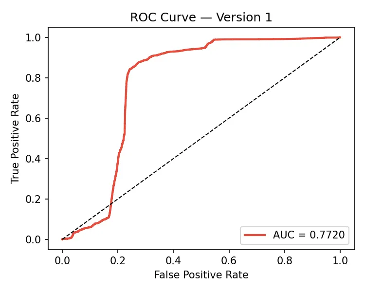
- AUC: 0.7720
- Precision (attack): 0.92
- Recall (attack): 0.62
The interesting part isn’t the accuracy. It’s the gap between precision and recall.
When the model says “this is an attack,” it’s right 92% of the time. But it only catches 62% of actual attacks. It misses more than a third of intrusions.
If you deployed this in a SOC, you’d have very few false alarms—but a lot of attacks slipping through undetected. For a red teamer, that’s a comfortable margin.
Version 2: The Counterintuitive Move — Use Less Data
Here’s where it gets interesting.
Instead of feeding all 38 quantitative features to the model, I compressed them using Principal Component Analysis (PCA) into just 12 components. The categorical variables stayed as-is.
Why 12? I applied the Kaiser criterion—keep only the components whose eigenvalue exceeds 1 (meaning they explain more variance than a single original variable). This is the standard statistical rule, not an arbitrary choice.
Eigenvalue analysis (first 15 of 38):
  PC 1: eigenvalue = 7.00   ← keep
  PC 2: eigenvalue = 4.89   ← keep
  PC 3: eigenvalue = 3.64   ← keep
  ...
  PC12: eigenvalue = 1.00   ← keep (barely)
  PC13: eigenvalue = 0.998  ← drop
12 components retain 76.26% of the total variance. We lose some information, but we also lose the noise and the multicollinearity between correlated features.
The pipeline becomes: Standardize → PCA → Concatenate with one-hot categoricals → Train.
# Compress 38 quantitative features → 12 principal components
pca = PCA(n_components=12)
X_pca_train = pca.fit_transform(X_num_train_scaled)

# Combine with one-hot encoded categoricals
X_train = pd.concat([X_pca_train_df, X_cat_train], axis=1)
# Result: 92 features (12 PC + 80 one-hot) instead of 118
The Results
Comparing Version 1 (all features) to Version 2 (PCA):
- Features: 118 → 92 (−26 features)
- Accuracy: 75.39% → 75.66% (stable)
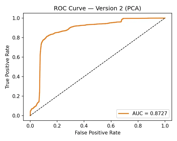
- AUC: 0.7720 → 0.8727 (+0.10)
The accuracy barely moved. But the AUC jumped by 0.10.
AUC (Area Under the Curve) evaluates the model across all possible decision thresholds. In practice, it answers: if you randomly pick one attack and one normal connection, how often does the model assign a higher attack probability to the attack?
A score of 0.5 means random guessing. A score of 1.0 means perfect separation. So when AUC increases, it means the model is much better at ranking attacks above normal traffic.
This is the counterintuitive finding: removing information improved discrimination. PCA stripped away the correlated noise between features like serror_rate and srv_serror_rate, letting the model focus on true anomalous signals.
What This Means for Detection (and Offense)
1. Your IDS is probably missing a third of attacks
Even with proper preprocessing, Logistic Regression catches ~63% of attacks on a structured dataset. Real network traffic is far messier. If an organization relies purely on signature or simple ML detection, significant blind spots exist.
2. Novel attacks break everything
The 14 unseen attack types in the test set are the primary reason accuracy caps at ~75%. The model cannot generalize to attack vectors it has never encountered. This is the fundamental challenge of supervised ML in security—and why adversarial thinking (red teaming) remains indispensable.
3. Feature engineering > model complexity
I used one of the simplest classifiers that exists—no deep neural nets, no XGBoost ensembles, no tuning. Yet with proper scaling and PCA, it achieved an AUC of 0.87. The bottleneck in detection is frequently data representation rather than raw model complexity.
4. Less data can mean better detection
If you are designing detection models, feeding every telemetry metric introduces noise and multicollinearity. Dimensionality reduction genuinely sharpens discrimination.
Red Team vs. ML — Testing My Own Attacks
Here’s where I put on my offensive hat.
I crafted 8 network connection records simulating real attacks I’ve performed or researched—Nmap scans, Hydra brute-force, SYN floods, Slowloris, and an interactive reverse shell callback.
I mapped what these attacks look like at the network transport level into KDD feature vectors and fed them to both models:
The Findings:
- Loud Attacks: Nmap scans, Hydra brute-force, and SYN floods were trivially flagged with 99%+ confidence by both models. Normal HTTP and DNS traffic was accurately classified.
- Slowloris (Slow HTTP DoS):
- Version 1 evaluated it as NORMAL with 99.9% confidence.
- Version 2 evaluated it as ATTACK at 72% confidence.
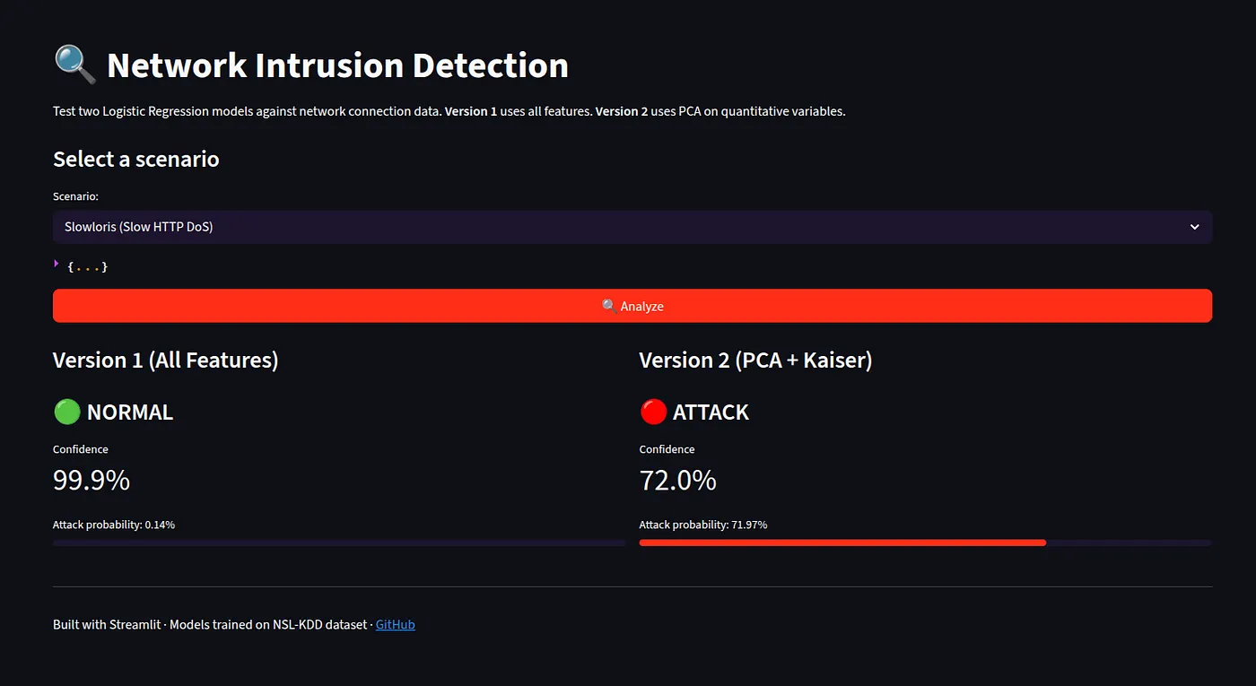
Why the difference? Version 1 evaluates each field in isolation: TCP traffic, HTTP port, connection established. In individual silos, Slowloris appears legitimate. But Version 2 compresses features into correlated behavioral clusters using PCA: a connection holding a socket open for hours while transmitting barely 20 bytes does not resemble normal traffic. V1 sees labels; V2 sees behavior.
- The Reverse Shell Blind Spot: Both models missed the reverse shell completely. At the network header level, an outbound TCP callback to a listener looks like any standard outbound session. Without deep payload inspection or endpoint telemetry, statistical network flows cannot detect the payload payload logic.
As a red teamer, the takeaway is clear: the model catches the loud, automated traffic and misses the quiet, deliberate post-exploitation.
Interactive Live Demo & Open Source Code
You can test arbitrary network connection parameters and simulate attacks directly in the interactive Streamlit app:
- 🚀 Live Demo: https://intrusion-detection-logistic-regression.streamlit.app/
- Manual Mode: Tweak all 41 features with interactive sliders.
- Preset Scenarios: One-click simulations for SYN floods, port scans, and smurf attacks.
- CSV Upload: Batch-evaluate connection captures.
Full Code & Reproduction
The complete training scripts, PCA pipeline, red team simulation scripts, and LaTeX whitepaper are available on GitHub:
- 📦 GitHub Repository: https://github.com/Haitam-lazaar/intrusion-detection-logistic-regression
git clone https://github.com/Haitam-lazaar/intrusion-detection-logistic-regression
cd intrusion-detection-logistic-regression
python3 -m venv venv && source venv/bin/activate
pip install -r requirements.txt
python src/version1.py          # Version 1: all 118 features
python src/version2.py          # Version 2: PCA dimensionality reduction
python src/redteam_test.py      # Red team attack test suite
streamlit run streamlit/app.py  # Interactive dashboard
Understanding detection internals—and exactly where statistical models fail—is fundamental to building more resilient defenses and executing more rigorous offensive assessments.